Tutorial 2 - Poisson GLM with Spike History and Coupling#
Run this tutorial yourself
Download this page as a Jupyter notebook (.ipynb) and run it locally.
This tutorial is an adaptation of JW Pillow’s material, presented at the Data Science and Data Skills for Neuroscientists short course at the SfN 2016 meeting.
This is an interactive tutorial designed to walk you through the steps of fitting an autoregressive Poisson GLM (i.e., a spiking GLM with spike-history) and a multivariate autoregressive Poisson GLM (i.e., a GLM with spike-history AND coupling between neurons).
(Data from Uzzell & Chichilnisky, 2004; see README.txt file in the /data_RGCs directory for details).
The dataset can be downloaded here:
The dataset is provided for tutorial purposes only, and should not be distributed or used for publication without express permission from EJ Chichilnisky (ej@stanford.edu).
Load and pre-process the data#
Below is a quick bit of data wrangling with pynapple that loads and temporally aligns the time series. The final result will be a TsGroup that contains the spike times from 4 RGC units, the corresponding spike counts as a TsdFrame, and a Tsd with the stimulus.
For more details on the pynapple objects and a step-by-step walkthrough of the pre-processing, see the first tutorial.
import matplotlib.pyplot as plt
import numpy as np
from nemos_tutorials import fetch_data, PALETTE, plot_counts, plot_design_matrix
import pynapple as nap
import jax
from scipy.io import loadmat

# enable float64 for precision
jax.config.update("jax_enable_x64", True)

data_paths = fetch_data("data_RGCs")

# Load spike times
spike_times = loadmat(data_paths["SpTimes.mat"], simplify_cells=True)["SpTimes"]
units = nap.TsGroup({i: nap.Ts(val) for i, val in enumerate(spike_times)})

# Load stimulus times and values
stim_times = loadmat(data_paths["stimtimes.mat"], simplify_cells=True)["stimtimes"]
stim = loadmat(data_paths["Stim.mat"], simplify_cells=True)["Stim"]
stimulus = nap.Tsd(stim_times, stim)

# Align time support
units = units.restrict(stimulus.time_support)

# Count the spikes
bin_size = stimulus.t[1] - stimulus.t[0]
counts = units.count(bin_size, stimulus.time_support)

# Re-sample the stimulus
stimulus = counts.value_from(stimulus, mode="before")
Compute and plot the cross-correlogram#
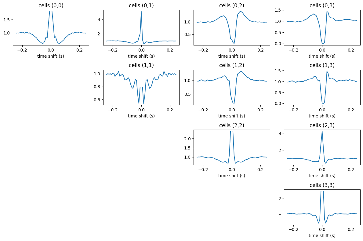
As a first step, let’s take a look at the cross-correlograms (CCGs), and let’s compute them via the pynapple functions compute_crosscorrelogram and compute_autocorrelogram.
# 30 bins matching the original tutorial
window_size_sec = 30 * bin_size

ccgs = nap.compute_crosscorrelogram(units, binsize=bin_size, windowsize=window_size_sec)
acgs = nap.compute_autocorrelogram(units, binsize=bin_size, windowsize=window_size_sec)

# drop acgs at t=0
acgs.loc[0] = np.nan

# plot the first 10 rows
ccgs.iloc[:10]
| 0 | 1 | 2 | ||||
|---|---|---|---|---|---|---|
| 1 | 2 | 3 | 2 | 3 | 3 | |
| -0.241878 | 0.987223 | 0.980394 | 0.976701 | 0.977630 | 0.976818 | 0.994896 |
| -0.233537 | 1.010966 | 0.987254 | 0.993758 | 0.972412 | 0.982707 | 1.008001 |
| -0.225196 | 1.003122 | 0.994846 | 0.993758 | 0.997966 | 1.006883 | 0.994026 |
| -0.216856 | 1.017537 | 1.001157 | 0.983163 | 1.017500 | 1.020366 | 1.015691 |
| -0.208515 | 1.007150 | 0.994846 | 0.993334 | 1.026732 | 1.034159 | 1.029064 |
| -0.200175 | 1.019869 | 0.972071 | 0.969285 | 0.993417 | 0.986272 | 1.011412 |
| -0.191834 | 1.014146 | 0.975090 | 0.962398 | 0.981643 | 0.987821 | 0.996300 |
| -0.183493 | 1.000790 | 0.976553 | 0.959750 | 0.978432 | 0.957446 | 0.981389 |
| -0.175153 | 0.988919 | 0.989266 | 0.984646 | 1.000375 | 1.003474 | 0.995631 |
| -0.166812 | 1.026441 | 1.010852 | 1.003399 | 1.025662 | 1.018042 | 1.000111 |
As you can see, the CCGs are stored in a pandas dataframe. Each column represents a pair of units, with the column name indicating the pair. Let’s plot them.
fig = plt.figure(figsize=[12,8])
for i in acgs.columns:
    plt.subplot(len(units), len(units), i*len(units) + i + 1)
    plt.title(f'cells ({i},{i})')
    plt.plot(acgs[i])
    plt.xlabel('time shift (s)')

for i, j in ccgs.columns:
    plt.subplot(len(units), len(units), i*len(units) + j + 1)
    plt.title(f'cells ({i},{j})')
    plt.plot(ccgs[i, j])
    plt.xlabel('time shift (s)')
plt.tight_layout()
plt.show()
Building the design matrix#
Let’s build a design matrix that uses as predictors the history of the stimulus (as in the first tutorial), and the spike count history of the neuron we are fitting. The last term will capture the autocorrelation structure of the spike count time series.
As before, we can use the NeMoS HistoryConv basis to capture the history effect of both predictors. One way to construct this is to create two basis, create the design matrices, and then concatenate them. An alternative and easier way to construct the same predictor in NeMoS is to use basis addition: adding two basis together result in a composite basis that concatenate design matrices.
import nemos as nmo

# match the original tutorial
cell_idx = 2
neuron_counts = counts[:, cell_idx]

# number of history time bins used for prediction
window_size_stim = 25
window_size_spk = 20

# Define the basis and specify labels to help tracking
# the component identity

# Basis for the stimulus
# (do not shift by 1 after convolve: stim_t is used as predictor of counts_t)
bas_stim = nmo.basis.HistoryConv(window_size_stim, conv_kwargs={"shift": False}, label="stim")

# Basis for the spike hist
# (shift after convolve: count_t is NOT used to predict count_t)
bas_spk = nmo.basis.HistoryConv(window_size_spk, label="spike")

# add
bas = bas_stim + bas_spk
bas
'(stim + spike)': AdditiveBasis(
    basis1='stim': HistoryConv(window_size=25, conv_kwargs={'shift': False}),
    basis2='spike': HistoryConv(window_size=20),
)
In a Jupyter environment, please rerun this cell to show the HTML representation or trust the notebook. On GitHub, the HTML representation is unable to render, please try loading this page with nbviewer.org.
Parameters
| label | '(stim + spike)' | |
| stim__conv_kwargs | {'shift': False} | |
| stim__label | 'stim' | |
| stim__window_size | 25 | |
| stim | 'stim': Histo...hift': False}) | |
| spike__conv_kwargs | {} | |
| spike__label | 'spike' | |
| spike__window_size | 20 | |
| spike | 'spike': Hist...indow_size=20) |
Once we have our additive basis, we can call compute feature passing the predictors in the correct order to get the full design matrix.
X = bas.compute_features(stimulus, neuron_counts)
X
/opt/hostedtoolcache/Python/3.12.13/x64/lib/python3.12/site-packages/pynapple/core/utils.py:198: UserWarning: Converting 'd' to numpy.array. The provided array was of type 'ArrayImpl'.
  warnings.warn(
/opt/hostedtoolcache/Python/3.12.13/x64/lib/python3.12/site-packages/pynapple/core/utils.py:198: UserWarning: Converting 'd' to numpy.array. The provided array was of type 'ArrayImpl'.
  warnings.warn(
Time (s)                   0       1       2       3       4  ...
--------------------  ------  ------  ------  ------  ------  -----
0.012510907499999998  nan     nan     nan     nan     nan     ...
0.0208515125          nan     nan     nan     nan     nan     ...
0.0291921175          nan     nan     nan     nan     nan     ...
0.0375327225          nan     nan     nan     nan     nan     ...
0.0458733275          nan     nan     nan     nan     nan     ...
0.0542139325          nan     nan     nan     nan     nan     ...
0.0625545375          nan     nan     nan     nan     nan     ...
...                                                           ...
1201.4182769225        -0.48   -0.48   -0.48    0.48    0.48  ...
1201.4266175275        -0.48   -0.48   -0.48   -0.48    0.48  ...
1201.4349581325        -0.48   -0.48   -0.48   -0.48   -0.48  ...
1201.4432987374998     -0.48   -0.48   -0.48   -0.48   -0.48  ...
1201.4516393425        -0.48   -0.48   -0.48   -0.48   -0.48  ...
1201.4599799475         0.48   -0.48   -0.48   -0.48   -0.48  ...
1201.4683205525         0.48    0.48   -0.48   -0.48   -0.48  ...
dtype: float64, shape: (144050, 45)
The total number of columns is 45, 25 columns capturing the stimulus history, and 20 for the spike history. The bookkeeping of which columns belong to which predictor may become messy, and bug-prone, especially for multiple high-dimensional predictors. Fortunately, the basis object takes care of the bookkeeping for us. Let’s see how to use the split_by_feature method to partition the design matrix into the two components and let’s plot them.
# Split by feature and return a dict with keys the basis label
split_dict = bas.split_by_feature(X, axis=1)

# Loop over the two predictors and print their shapes
for key, Xi in split_dict.items():
    print(key, Xi.shape)
stim (144050, 25)
spike (144050, 20)
As in the first tutorial, we build the design with the HistoryConv basis, which means each predictor’s columns come in the reverse order from the original notebook. This doesn’t change the model — see the note there for why — so we keep NeMoS’ natural column order and flip only when plotting the filters.
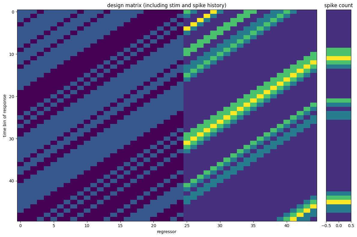
Now let’s plot the design. Let’s remember that NeMoS performs a convolution in mode valid, and append NaNs to preserve the total number of samples, which naturally maintains the temporal alignment with the predicted variable.
For display we reorder each feature’s columns so the most lagged lag comes first
(see plot_design_matrix), reusing the split_dict from above and skipping the
NaN-padded burn-in.
# skip the first NaNs and zoom into a 50-bin window
rows = slice(window_size_stim, window_size_stim + 50)
plot_design_matrix(
    split_dict,
    counts=neuron_counts,
    rows=rows,
    title="design matrix (including stim and spike history)",
)
plt.tight_layout()
plt.show()
Fit a single-neuron GLM with spike-history#
Now we are ready to fit our Poisson GLM. Let’s fit two models: a model that uses the stimulus as predictor, and one that uses both the stimulus and the spike history.
We can take advantage of the basis bookkeeping again to split the design matrix.
model_stim_only = nmo.glm.GLM(solver_name="BFGS")
model_stim_spk =  nmo.glm.GLM(solver_name="BFGS")

model_stim_only.fit(bas.split_by_feature(X, axis=1)["stim"], neuron_counts)
model_stim_spk.fit(X, neuron_counts)
GLM(
    observation_model=PoissonObservations(),
    inverse_link_function=exp,
    regularizer=UnRegularized(),
    solver_name='BFGS'
)
In a Jupyter environment, please rerun this cell to show the HTML representation or trust the notebook. On GitHub, the HTML representation is unable to render, please try loading this page with nbviewer.org.
Parameters
| observation_model | PoissonObservations() | |
| inverse_link_function | <function exp...x7f66e0dae660> | |
| regularizer | UnRegularized() | |
| solver_name | 'BFGS' | |
| solver_kwargs | {} | |
| regularizer_strength | None |
Fitted attributes
| Name | Type | Value |
|---|---|---|
| aux_ | NoneType | None |
| coef_ | ArrayImpl[float64](45,) | Array([ 3.937...dtype=float64) |
| dof_resid_ | ArrayImpl[float64](1,) | Array([144049...dtype=float64) |
| intercept_ | ArrayImpl[float64](1,) | Array([-1.282...dtype=float64) |
| scale_ | ArrayImpl[float64](1,) | Array([1.], dtype=float64) |
| solver_state_ | OptimistixAdapterState | OptimistixAda...k_bool[] ) ) |
Both filter plots below need the weights reordered the same way, so let’s define a small helper that does the reordering and draws a single filter onto a given axis.
def plot_filter(ax, lags, weights, title, **kwargs):
    # NeMoS' HistoryConv returns the weights with the most recent lag first, so we
    # flip them with [::-1] to align with lag time and match the original notebook.
    ax.plot(lags, weights[::-1], marker="o", **kwargs)
    ax.set_title(title)
    ax.set_xlabel("time before spike (s)")
    ax.set_ylabel("weight")
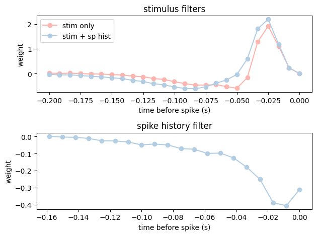
And finally, let’s plot and compare the filters.
# split coefficients for composite model
coef_dict = bas.split_by_feature(model_stim_spk.coef_, axis=0)

f, (ax1, ax2) = plt.subplots(2,1)
lags_stim = np.arange(-1 * window_size_stim + 1,1) * bin_size
lags_spk = np.arange(-1 * window_size_spk + 1,1) * bin_size

plot_filter(ax1, lags_stim, model_stim_only.coef_, "stimulus filters", color=PALETTE[0], label="stim only")
plot_filter(ax1, lags_stim, coef_dict["stim"], "stimulus filters", color=PALETTE[1], label="stim + sp hist")
ax1.legend(loc="upper left")

plot_filter(ax2, lags_spk, coef_dict["spike"], "spike history filter", color=PALETTE[1])

plt.tight_layout()
plt.show()
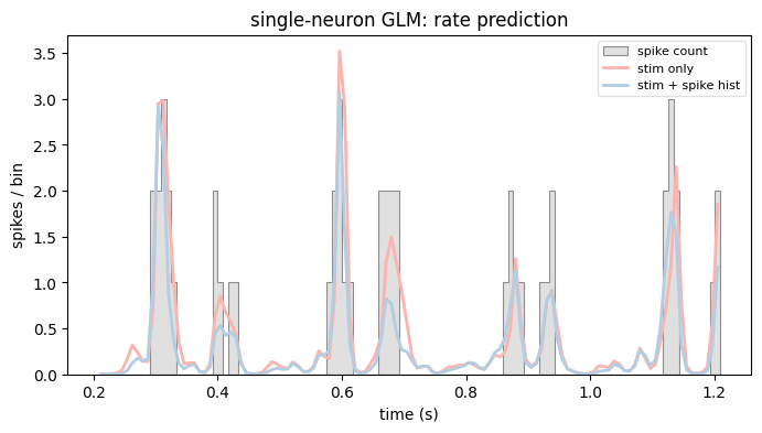
Adding the spike history sharpens the prediction. Let’s look at the predicted rate of both models against the observed spike counts. We reuse the plot_counts helper from the first tutorial, now shared via the nemos_tutorials package.
# Stimulus-only model is fit on the stim sub-block of the design matrix.
X_stim = bas.split_by_feature(X, axis=1)["stim"]

rate_stim_only = model_stim_only.predict(X_stim)
rate_stim_spk = model_stim_spk.predict(X)

# Pick a 1-second window starting after the NaN-padded history bins.
t0 = rate_stim_spk.dropna().t[0]
ep = (t0, t0 + 1)

plot_counts(
    neuron_counts,
    ep,
    [
        (rate_stim_only, "stim only"),
        (rate_stim_spk, "stim + spike hist"),
    ],
    title="single-neuron GLM: rate prediction",
    ylabel="spikes / bin",
)
plt.show()
/opt/hostedtoolcache/Python/3.12.13/x64/lib/python3.12/site-packages/pynapple/core/utils.py:198: UserWarning: Converting 'd' to numpy.array. The provided array was of type 'ArrayImpl'.
  warnings.warn(
Fit coupled GLM for multiple-neuron responses#
Instead of using the spike history of the fitted neuron only (auto-correlation filter), we will learn the functional connectivity by including the spike history of all the other neurons. In NeMoS this is trivial, since every basis is applied in a vectorized way over any extra axis:
If
xis 1D, thenbasis.compute_features(x)will return a \((n_{\text{samples}}, n_{\text{basis}})\) array.If
xis ND with shape \((n_{\text{samples}}, i_1, \dots, i_{n-1})\), then the output will have shape \((n_{\text{samples}}, n_{\text{basis}}\cdot \prod_{j=1}^{n-1} i_j )\).
Therefore, including all counts as predictors follows exactly the same syntax as the single count array case. The only caveat concerns the basis bookkeeping: we build the coupled design from a freshly constructed basis, bas_coupling, leaving the single-neuron bas untouched.
# Let's re-create the basis (see admonition below for why)
bas_coupling = bas_stim + bas_spk

X_coupling = bas_coupling.compute_features(stimulus, counts)
X_coupling
/opt/hostedtoolcache/Python/3.12.13/x64/lib/python3.12/site-packages/pynapple/core/utils.py:198: UserWarning: Converting 'd' to numpy.array. The provided array was of type 'ArrayImpl'.
  warnings.warn(
/opt/hostedtoolcache/Python/3.12.13/x64/lib/python3.12/site-packages/pynapple/core/utils.py:198: UserWarning: Converting 'd' to numpy.array. The provided array was of type 'ArrayImpl'.
  warnings.warn(
Time (s)                   0       1       2       3       4  ...
--------------------  ------  ------  ------  ------  ------  -----
0.012510907499999998  nan     nan     nan     nan     nan     ...
0.0208515125          nan     nan     nan     nan     nan     ...
0.0291921175          nan     nan     nan     nan     nan     ...
0.0375327225          nan     nan     nan     nan     nan     ...
0.0458733275          nan     nan     nan     nan     nan     ...
0.0542139325          nan     nan     nan     nan     nan     ...
0.0625545375          nan     nan     nan     nan     nan     ...
...                                                           ...
1201.4182769225        -0.48   -0.48   -0.48    0.48    0.48  ...
1201.4266175275        -0.48   -0.48   -0.48   -0.48    0.48  ...
1201.4349581325        -0.48   -0.48   -0.48   -0.48   -0.48  ...
1201.4432987374998     -0.48   -0.48   -0.48   -0.48   -0.48  ...
1201.4516393425        -0.48   -0.48   -0.48   -0.48   -0.48  ...
1201.4599799475         0.48   -0.48   -0.48   -0.48   -0.48  ...
1201.4683205525         0.48    0.48   -0.48   -0.48   -0.48  ...
dtype: float64, shape: (144050, 105)
Why are we re-defining the basis?
Every call to compute_features inspects the shape of its inputs and stores it on the basis, so that a later split_by_feature knows how to carve the design matrix (or the coefficient vector) back into per-feature blocks of the right shape. This stored shape is overwritten on each call. If we reused the same bas object to build the coupled design, its spike block would be reshaped for 4 neurons, and we would no longer be able to split the single-neuron model’s coefficients with it. Building the coupled design from a fresh bas_coupling keeps both models’ bookkeeping intact.
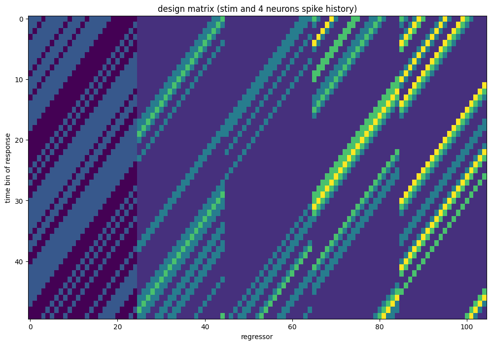
Now the number of columns is 105 = 25 + 20 * 4, where 4 is the number of units.
Again, we can split this design in interpretable components.
split_coupling = bas_coupling.split_by_feature(X_coupling, axis=1)
print("Keys:", split_coupling.keys())
Keys: dict_keys(['stim', 'spike'])
But this time, the spike component of the design matrix is conveniently reshaped as (n_samples, n_neurons, n_basis_funcs), one spike-history block per neuron.
print("(n_samples, n_neurons, n_basis_funcs): ", split_coupling["spike"].shape)
(n_samples, n_neurons, n_basis_funcs): (144050, 4, 20)
As in the single-neuron case, the HistoryConv columns come in the reverse order from the original notebook, and we keep NeMoS’ order here too (see the first tutorial for why). The design is already a single 2D matrix (n_samples, n_regressors), so we can use it as is.
Let’s plot it.
# same per-feature reordering, now on the coupled split (the spike block is 3D)
plot_design_matrix(
    split_coupling,
    rows=slice(window_size_stim, window_size_stim + 50),
    title="design matrix (stim and 4 neurons spike history)",
)
plt.show()
Finally, let’s fit the coupled model.
model_coupled =  nmo.glm.GLM(solver_name="BFGS")
model_coupled.fit(X_coupling, neuron_counts)
GLM(
    observation_model=PoissonObservations(),
    inverse_link_function=exp,
    regularizer=UnRegularized(),
    solver_name='BFGS'
)
In a Jupyter environment, please rerun this cell to show the HTML representation or trust the notebook. On GitHub, the HTML representation is unable to render, please try loading this page with nbviewer.org.
Parameters
| observation_model | PoissonObservations() | |
| inverse_link_function | <function exp...x7f66e0dae660> | |
| regularizer | UnRegularized() | |
| solver_name | 'BFGS' | |
| solver_kwargs | {} | |
| regularizer_strength | None |
Fitted attributes
| Name | Type | Value |
|---|---|---|
| aux_ | NoneType | None |
| coef_ | ArrayImpl[float64](105,) | Array([ 4.777...dtype=float64) |
| dof_resid_ | ArrayImpl[float64](1,) | Array([144049...dtype=float64) |
| intercept_ | ArrayImpl[float64](1,) | Array([-1.264...dtype=float64) |
| scale_ | ArrayImpl[float64](1,) | Array([1.], dtype=float64) |
| solver_state_ | OptimistixAdapterState | OptimistixAda...k_bool[] ) ) |
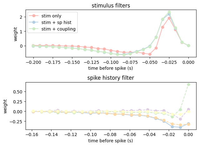
And let’s compare all the results.
coef_coupling_dict = bas_coupling.split_by_feature(model_coupled.coef_, axis=0)

f, (ax1, ax2) = plt.subplots(2,1)
lags_stim = np.arange(-1 * window_size_stim + 1,1) * bin_size
lags_spk = np.arange(-1 * window_size_spk + 1,1) * bin_size

plot_filter(ax1, lags_stim, model_stim_only.coef_, "stimulus filters", color=PALETTE[0], label="stim only")
plot_filter(ax1, lags_stim, coef_dict["stim"], "stimulus filters", color=PALETTE[1], label="stim + sp hist")
plot_filter(ax1, lags_stim, coef_coupling_dict["stim"], "stimulus filters", color=PALETTE[2], label="stim + coupling")
ax1.legend(loc="upper left")

plot_filter(ax2, lags_spk, coef_dict["spike"], "spike history filter", color=PALETTE[1])
for i, coef in enumerate(coef_coupling_dict["spike"]):
    plot_filter(ax2, lags_spk, coef, "spike history filter", ls="--", color=PALETTE[2+i])

plt.tight_layout()

plt.show()
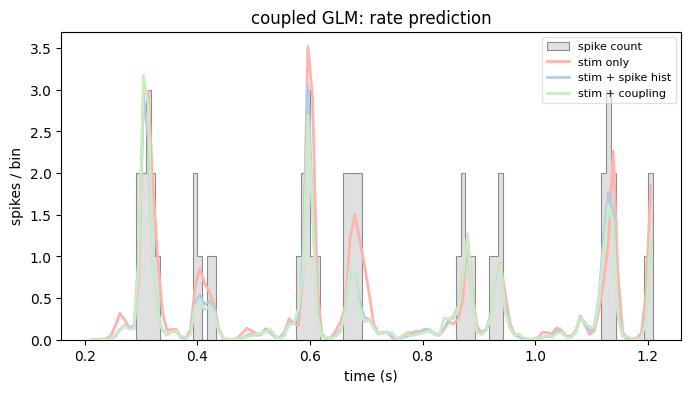
And, as before, let’s compare the predicted rates of all three models on the same window we used above.
rate_coupled = model_coupled.predict(X_coupling)

plot_counts(
    neuron_counts,
    ep,
    [
        (rate_stim_only, "stim only"),
        (rate_stim_spk, "stim + spike hist"),
        (rate_coupled, "stim + coupling"),
    ],
    title="coupled GLM: rate prediction",
    ylabel="spikes / bin",
)
plt.show()
/opt/hostedtoolcache/Python/3.12.13/x64/lib/python3.12/site-packages/pynapple/core/utils.py:198: UserWarning: Converting 'd' to numpy.array. The provided array was of type 'ArrayImpl'.
  warnings.warn(
Comparing the models#
The filters and rate traces show that each added predictor changes the fit, but how much do we actually gain? Let’s quantify it with two complementary metrics: the single-spike information (how many bits per spike the model buys us over a constant-rate baseline) and the AIC (which rewards fit but charges for extra parameters). Both build on the same quantity — the total log-likelihood of each fitted model — so let’s compute that first.
One thing to be careful about: the convolution pads the start of each design with NaNs. Rather than hardcoding the window length, let’s let the data tell us which bins are valid. Calling dropna on a design returns its non-NaN time support, and since all three designs share the same padding (the stimulus history is the longest window), any of them defines the common valid_epochs.
valid_epochs = X.dropna().time_support
Now we can restrict all the time series to valid_epochs and evaluate each model on the same bins. We keep the (model, design) pair for each fit in a dict, since we’ll reuse both below.
counts_valid = neuron_counts.restrict(valid_epochs)

# (model, design matrix) for each of the three fits
fits = {
    "stim only": (model_stim_only, X_stim.restrict(valid_epochs)),
    "stim + spike hist": (model_stim_spk, X.restrict(valid_epochs)),
    "stim + coupling": (model_coupled, X_coupling.restrict(valid_epochs)),
}
By default, score returns the mean log-likelihood per sample. Here we want the total, so we pass aggregate_sample_scores=np.sum to sum the per-sample scores instead of averaging them.
log_likelihood = {
    name: model.score(design, counts_valid, aggregate_sample_scores=np.sum)
    for name, (model, design) in fits.items()
}
Single-spike information#
A raw log-likelihood is hard to read on its own, so we compare each model against a baseline that ignores everything and just fires at the constant mean rate. The difference between the two log-likelihoods, divided by the number of spikes and converted to base 2, is the single-spike information: the bits per spike we gain by knowing the model’s rate rather than the mean rate (Brenner et al., “Synergy in a Neural Code”, Neural Comp 2000).
The baseline is a homogeneous Poisson model firing at the mean spike count. It is not a fitted GLM, so we evaluate its log-likelihood directly on the observation model.
n_samples = counts_valid.shape[0]
n_spikes = counts_valid.sum()

# Homogeneous Poisson baseline: constant rate = mean spike count.
mean_rate = np.mean(counts_valid) * np.ones(n_samples)
ll_null = model_stim_spk.observation_model.log_likelihood(
    counts_valid.d,
    mean_rate,
    aggregate_sample_scores=np.sum
)

print("empirical single-spike information:\n-----------------------------------")
for name, ll in log_likelihood.items():
    ss_info = float((ll - ll_null) / n_spikes / np.log(2))
    print(f"{name:<18}: {ss_info:.2f} bits/sp")
empirical single-spike information:
-----------------------------------
stim only         : 1.11 bits/sp
stim + spike hist : 1.19 bits/sp
stim + coupling   : 1.20 bits/sp
Each added filter buys a bit more information per spike, with the biggest jump coming from the spike history.
AIC#
Single-spike information rewards a model for fitting the spikes but says nothing about how many parameters that fit cost. The Akaike Information Criterion charges for complexity,
where \(k\) is the number of free parameters and lower is better. We read \(k\) straight off each fitted model: its filter weights plus the intercept.
def count_pars(model):
    """Number of free parameters: filter weights plus intercept."""
    return model.coef_.size + model.intercept_.size

aics = {
    name: float(-2 * log_likelihood[name] + 2 * count_pars(model))
    for name, (model, _) in fits.items()
}

for name, aic in aics.items():
    print(f"AIC  {name:<18}: {aic:.1f}")

winner = min(aics, key=aics.get)
print(f"\nAIC favors the '{winner}' model.")
AIC  stim only         : 150537.2
AIC  stim + spike hist : 144955.2
AIC  stim + coupling   : 143848.3

AIC favors the 'stim + coupling' model.
Both metrics agree: the spike-history and coupling terms each add structure the stimulus alone cannot capture — the spike-history filter accounts for the cell’s own refractoriness and bursting, while the coupling filters absorb shared variability from the rest of the population — and the improvement in fit more than pays for the extra parameters.
The whole pipeline, side by side
Here is the entire path from the raw .mat files to a fitted coupled GLM, in both stacks. Same model, same result (the single-spike information and AIC above match the original to the second decimal) — the only difference is how much bookkeeping you write by hand.
pynapple + NeMoS:
import numpy as np, pynapple as nap, nemos as nmo
from scipy.io import loadmat
from nemos_tutorials import fetch_data

paths = fetch_data("data_RGCs")

# load, align, count, resample
units = nap.TsGroup({i: nap.Ts(v) for i, v in
                     enumerate(loadmat(paths["SpTimes.mat"], simplify_cells=True)["SpTimes"])})
stimulus = nap.Tsd(loadmat(paths["stimtimes.mat"], simplify_cells=True)["stimtimes"],
                   loadmat(paths["Stim.mat"], simplify_cells=True)["Stim"])
units = units.restrict(stimulus.time_support)
bin_size = stimulus.t[1] - stimulus.t[0]
counts = units.count(bin_size, stimulus.time_support)
stimulus = counts.value_from(stimulus, mode="before")

# design (stim history + every neuron's spike history) and fit
bas = (nmo.basis.HistoryConv(25, conv_kwargs={"shift": False}, label="stim")
       + nmo.basis.HistoryConv(20, label="spike"))
X = bas.compute_features(stimulus, counts)
model = nmo.glm.GLM(solver_name="BFGS").fit(X, counts[:, 2])

# recover the filters, already shaped and labelled
filters = bas.split_by_feature(model.coef_, axis=0)
stim_filter = filters["stim"]    # (25,)
spk_filters = filters["spike"]   # (4, 20)  -> one row per neuron
NumPy + statsmodels (the original):
import numpy as np, statsmodels.api as sm
from scipy.io import loadmat
from scipy.linalg import hankel

stim = np.squeeze(loadmat("data_RGCs/Stim.mat")["Stim"])
stim_times = np.squeeze(loadmat("data_RGCs/stimtimes.mat")["stimtimes"])
spikes = [np.squeeze(x) for x in np.squeeze(loadmat("data_RGCs/SpTimes.mat")["SpTimes"])]
num_cells, dt, n = len(spikes), stim_times[1] - stim_times[0], stim.size
cell_idx, ntfilt, nthist = 2, 25, 20

# bin spikes on a grid anchored at zero
binned = np.stack([np.histogram(s, np.arange(n + 1) * dt)[0] for s in spikes], axis=1)
y = binned[:, cell_idx]

# stimulus design via hankel (manual zero-padding)
padded_stim = np.hstack((np.zeros(ntfilt - 1), stim))
Xstim = hankel(padded_stim[:-ntfilt + 1], stim[-ntfilt:])

# spike-history design for every neuron, shifted one bin back so a bin can't predict itself
Xspk = np.zeros((n, nthist, num_cells))
for j in range(num_cells):
    padded = np.hstack((np.zeros(nthist), binned[:-1, j]))
    Xspk[:, :, j] = hankel(padded[:-nthist + 1], padded[-nthist:])
Xspk = Xspk.reshape(n, -1, order="F")

# concatenate, add an intercept column, fit
X = np.hstack((np.ones((n, 1)), Xstim, Xspk))
model = sm.GLM(y, X, family=sm.families.Poisson()).fit(max_iter=100, tol=1e-6, tol_criterion="params")

# recover the filters by hand: slice past the intercept, and un-flatten the
# coupling block with the same order="F" used to build it (then transpose)
params = model.params
stim_filter = params[1:ntfilt + 1]                                         # (25,)
spk_filters = params[ntfilt + 1:].reshape(nthist, num_cells, order="F").T  # (4, 20)
The pynapple + NeMoS version is roughly half the lines — and that is despite the NumPy side being written in its most compressed form. But the line count is the least of it. The manual indexing ([:-ntfilt+1], the [:-1] one-bin shift, order="F", the intercept slice) is bookkeeping you have to carry by hand, and it only gets harder — both to write correctly and to read — as the model design grows more complex. The pynapple + NeMoS version avoids it entirely, which pays off in three ways:
Readability. Each line is practically self-documenting. Handed to a collaborator,
units.count(bin_size)needs no explanation, whereashankel(padded[:-nthist+1], padded[-nthist:])needs a paragraph.Generalization. The same syntax scales with the problem.
compute_featuresbuilds the design matrix identically for one predictor or many; thepynapplepreprocessing is the same for a single signal or a whole population; the GLM call is unchanged across model configurations.Fewer opportunities for bugs. There are no hand-written indices to get wrong, and index arithmetic is notoriously prone to off-by-one mistakes — the kind that don’t raise an error, they just quietly shift your filter by a bin.