Tutorial 5 - MAP Decoding#
Run this tutorial yourself
Download this page as a Jupyter notebook (.ipynb) and run it locally.
This tutorial is an adaptation of JW Pillow’s material, presented at the Data Science and Data Skills for Neuroscientists short course at the SfN 2016 meeting.
Introduction#
So far we have been doing encoding: given a stimulus, predict the spikes. Here we flip the direction and perform decoding: given the spikes, recover the variable that drove them.
In this example the variable being decoded is the visual stimulus; however, the same approach can be used to decode any other variable, including behavioral covariates such as the animal’s position or head direction. As long as the variable is encoded in the neural activity, we should be able to decode it from the spikes.
Notation#
We record over \(T\) time bins. The observed activity is
the spike counts in each bin (or, for a Gaussian observation model, a real-valued activity in \(\mathbb{R}^{T}\)). The variable we decode is
with \(T\) samples and \(D\) the dimensionality of the stimulus. In this notebook the stimulus is a one-dimensional binary white noise, so \(D = 1\) and each sample takes one of two values:
Decoding asks which \(\mathbf{s}\) most plausibly produced the observed \(\mathbf{y}\), using the fitted GLM as the forward model that links the two.
The MAP decoding framework#
Decoding is naturally framed as a Bayesian inference problem. We want the posterior \(P(\mathbf{s} \mid \mathbf{y})\) — how plausible each candidate stimulus is after seeing the spikes — and Bayes’ theorem builds it from two pieces:
The likelihood \(P(\mathbf{y} \mid \mathbf{s})\) is the observation model: how probable the recorded spike train is under a candidate stimulus. This is exactly the encoding GLM we fitted in the previous tutorials, now read in the other direction — we hold the spikes fixed and vary \(\mathbf{s}\).
The prior \(P(\mathbf{s})\) encodes our hypothesis about the stimulus before seeing any spikes: which stimuli we consider plausible a priori. Here we have no specific template in mind, only a structural belief — that the stimulus changes gradually rather than jumping erratically from one frame to the next. We capture this with a Gaussian that penalizes large jumps between consecutive frames — a smoothness prior — with precision (inverse covariance) matrix \(C^{-1}\):
Maximizing the posterior is equivalent to minimizing its negative log, which gives us the MAP objective:
We minimize this with a standard gradient-based optimizer (L-BFGS-B), respecting the physical bounds of the stimulus.
Load and pre-process the data#
The pre-processing is identical to the earlier tutorials: we load the RGC data, align the time supports, bin the spikes, and resample the stimulus. See Tutorial 1 for a step-by-step walkthrough.
import jax
jax.config.update("jax_enable_x64", True)

import matplotlib.pyplot as plt
import numpy as np
from scipy.io import loadmat

import pynapple as nap
import nemos as nmo
from nemos_tutorials import fetch_data, PALETTE

data_paths = fetch_data("data_RGCs")

# Load and wrap spike times
spike_times = loadmat(data_paths["SpTimes.mat"], simplify_cells=True)["SpTimes"]
units = nap.TsGroup({i: nap.Ts(val) for i, val in enumerate(spike_times)})

# Load and wrap stimulus
stim_times = loadmat(data_paths["stimtimes.mat"], simplify_cells=True)["stimtimes"]
stim = loadmat(data_paths["Stim.mat"], simplify_cells=True)["Stim"]
stimulus = nap.Tsd(stim_times, stim)

# Align, count, resample
units = units.restrict(stimulus.time_support)
bin_size = stimulus.t[1] - stimulus.t[0]
counts = units.count(bin_size, stimulus.time_support)
stimulus = counts.value_from(stimulus, mode="before")

cell_idx = 2
neuron_counts = counts[:, cell_idx]
Train / test split#
We set aside the first quarter of the recording as training data and reserve a short window of 50 bins immediately after it as the test window we will decode.
n_train = int(stimulus.size * (1 / 4))
n_test = 50
window_size_stim = 20

# The test window starts after the training data, offset by the filter length
# so that the design matrix has no NaN-padded rows in the test window.
n_test_start = n_train + window_size_stim - 1
n_test_stop  = n_test_start + n_test

y_test = neuron_counts[n_test_start:n_test_stop]
Fit the forward models#
Decoding requires a forward model. We fit two: a stimulus-only Poisson GLM (same as Tutorial 1) and an augmented GLM that also captures spike-history and coupling (Tutorial 2). We will decode with both and compare.
Stimulus-only GLM#
basis_stim = nmo.basis.HistoryConv(window_size_stim, label="stim", conv_kwargs={"shift": False})
X_stim = basis_stim.compute_features(stimulus[:n_train])
y_train = neuron_counts[:n_train]

glm_stim = nmo.glm.GLM(observation_model="Poisson")
glm_stim.fit(X_stim, y_train)
glm_stim
/opt/hostedtoolcache/Python/3.12.13/x64/lib/python3.12/site-packages/pynapple/core/utils.py:198: UserWarning: Converting 'd' to numpy.array. The provided array was of type 'ArrayImpl'.
  warnings.warn(
GLM(
    observation_model=PoissonObservations(),
    inverse_link_function=exp,
    regularizer=UnRegularized(),
    solver_name='LBFGS'
)
In a Jupyter environment, please rerun this cell to show the HTML representation or trust the notebook. On GitHub, the HTML representation is unable to render, please try loading this page with nbviewer.org.
Parameters
| observation_model | PoissonObservations() | |
| inverse_link_function | <function exp...x7fbaaef54720> | |
| regularizer | UnRegularized() | |
| solver_name | 'LBFGS' | |
| solver_kwargs | {} | |
| regularizer_strength | None |
Fitted attributes
| Name | Type | Value |
|---|---|---|
| aux_ | NoneType | None |
| coef_ | ArrayImpl[float64](20,) | Array([ 0.003...dtype=float64) |
| dof_resid_ | ArrayImpl[float64](1,) | Array([36011.], dtype=float64) |
| intercept_ | ArrayImpl[float64](1,) | Array([-1.924...dtype=float64) |
| scale_ | ArrayImpl[float64](1,) | Array([1.], dtype=float64) |
| solver_state_ | OptimistixAdapterState | OptimistixAda...k_bool[] ) ) |
GLM with spike history and coupling#
window_size_spk = 20

basis_spk  = nmo.basis.HistoryConv(window_size_spk,  label="spike")
basis_stim_spk = basis_stim + basis_spk

X_stim_spk = basis_stim_spk.compute_features(stimulus[:n_train], counts[:n_train])
glm_stim_spk = nmo.glm.GLM(observation_model="Poisson", solver_name="BFGS")
glm_stim_spk.fit(X_stim_spk, y_train)
glm_stim_spk
/opt/hostedtoolcache/Python/3.12.13/x64/lib/python3.12/site-packages/pynapple/core/utils.py:198: UserWarning: Converting 'd' to numpy.array. The provided array was of type 'ArrayImpl'.
  warnings.warn(
/opt/hostedtoolcache/Python/3.12.13/x64/lib/python3.12/site-packages/pynapple/core/utils.py:198: UserWarning: Converting 'd' to numpy.array. The provided array was of type 'ArrayImpl'.
  warnings.warn(
GLM(
    observation_model=PoissonObservations(),
    inverse_link_function=exp,
    regularizer=UnRegularized(),
    solver_name='BFGS'
)
In a Jupyter environment, please rerun this cell to show the HTML representation or trust the notebook. On GitHub, the HTML representation is unable to render, please try loading this page with nbviewer.org.
Parameters
| observation_model | PoissonObservations() | |
| inverse_link_function | <function exp...x7fbaaef54720> | |
| regularizer | UnRegularized() | |
| solver_name | 'BFGS' | |
| solver_kwargs | {} | |
| regularizer_strength | None |
Fitted attributes
| Name | Type | Value |
|---|---|---|
| aux_ | NoneType | None |
| coef_ | ArrayImpl[float64](100,) | Array([ 6.465...dtype=float64) |
| dof_resid_ | ArrayImpl[float64](1,) | Array([36011.], dtype=float64) |
| intercept_ | ArrayImpl[float64](1,) | Array([-1.251...dtype=float64) |
| scale_ | ArrayImpl[float64](1,) | Array([1.], dtype=float64) |
| solver_state_ | OptimistixAdapterState | OptimistixAda...k_bool[] ) ) |
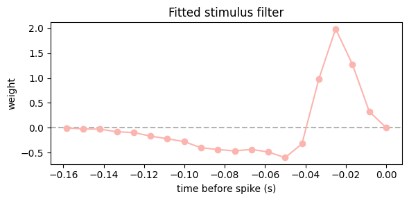
Let’s visualize the fitted stimulus filter from the simpler model.
lags = np.arange(-window_size_stim + 1, 1) * bin_size

fig, ax = plt.subplots(figsize=(6, 3))
ax.axhline(0, color="0.7", linestyle="--")
# reverse the coef to match original convention
# (see tutorial 1) for details
ax.plot(lags, glm_stim.coef_[::-1], "o-", color=PALETTE[0])
ax.set_title("Fitted stimulus filter")
ax.set_xlabel("time before spike (s)")
ax.set_ylabel("weight")
plt.tight_layout()
plt.show()
Define the smoothness prior#
For the prior \(P(\mathbf{s})\) we use a Gaussian with a first-difference precision matrix: it penalizes \(\sum_i (s_{i+1} - s_i)^2\), discouraging large jumps between consecutive frames and thus encouraging a smooth decoded stimulus. This is the same penalty we built by hand in Tutorial 3+4.
The first-difference operator \(D\) has shape \((n-1)\times n\) and satisfies \((D\mathbf{s})_i = s_{i+1} - s_i\). The smoothing precision matrix is \(C^{-1} = \lambda\, D^\top D\). We set \(\lambda\) to the empirical variance of the stimulus so that the prior scale matches the data.
from scipy.sparse import diags

# First-difference operator D, shape (n_test-1, n_test)
main_diag  = np.ones(n_test - 1)
upper_diag = -np.ones(n_test - 1)
Dx1 = diags(
    diagonals=[main_diag, upper_diag],
    offsets=[0, 1],
    shape=(n_test - 1, n_test),
).toarray()

# Precision matrix C^{-1} = lambda * D^T D
Dx   = Dx1.T @ Dx1
lam  = float(np.var(stimulus))   # scale to the stimulus variance
Cinv = lam * Dx
Why use the stimulus variance as \(\lambda\)?
The prior covariance is \(C = (C^{-1})^{-1} = (\lambda D^\top D)^{-1}\). Choosing \(\lambda = \mathrm{Var}(s)\) puts the prior’s marginal standard deviation in the same ballpark as the observed stimulus fluctuations — a reasonable, weakly informative default that avoids both over-smoothing and an essentially flat prior.
MAP objective functions#
The MAP objective couples the forward model to the prior. For each candidate stimulus \(\mathbf{s}\) we:
Pad with zeros to give the filter a burn-in period (so the convolution has no edge artifacts at the start of the test window).
Build the design matrix via the basis’s
compute_features.Evaluate the negative log-likelihood of the fitted GLM at the test spike counts.
Add the prior penalty \(\frac{1}{2}\mathbf{s}^\top C^{-1} \mathbf{s}\).
def map_objective_stim(pred_stim, glm, basis, y_test, Cinv):
    """MAP objective for the stimulus-only GLM."""
    n_t = glm.coef_.shape[0]

    # Pad with zeros so the filter has a full burn-in before the test window.
    xx = np.concatenate([np.zeros(n_t * 2), pred_stim])

    # Build design matrix and keep only the test-window rows. Reverse the
    # columns to match the convention used when the model was fitted.
    X_pred = basis.compute_features(xx)
    X_pred = X_pred[-pred_stim.shape[0]:]

    # Negative log-likelihood under the fitted GLM.
    predicted_rate = glm.predict(X_pred)
    nll = glm._observation_model._negative_log_likelihood(
        y_test.values, predicted_rate, aggregate_sample_scores=np.sum
    )

    # Add prior penalty.
    return float(nll) + 0.5 * pred_stim @ Cinv @ pred_stim
The second objective additionally conditions on the actual spike counts observed during the test window. Since the coupled GLM uses spike history as a predictor, passing the real counts in gives it more information and should yield a better decode.
def map_objective_stim_spk(pred_stim, glm, basis, y_test, Cinv, counts_test):
    """MAP objective for the GLM with spike history and coupling."""
    n_t = max(basis["stim"].window_size, basis["spike"].window_size)

    # Pad stimulus and spike counts with zeros for the burn-in period.
    xx = np.concatenate([np.zeros(n_t * 2), pred_stim])
    ss = np.concatenate([
        np.zeros((n_t * 2, counts_test.shape[1])),
        np.asarray(counts_test),
    ])

    # Build design matrix and keep only the test-window rows.
    X_pred = basis.compute_features(xx, ss)
    X_pred = X_pred[-pred_stim.shape[0]:]

    # Negative log-likelihood under the fitted GLM.
    predicted_rate = glm.predict(X_pred)
    nll = glm._observation_model._negative_log_likelihood(
        y_test.values, predicted_rate, aggregate_sample_scores=np.sum
    )

    return float(nll) + 0.5 * pred_stim @ Cinv @ pred_stim
Why pad with zeros?
HistoryConv looks back window_size bins to form each row of the design matrix. Without any burn-in, the very first rows of the test window would be fed zeros (or NaNs) for the stimulus that “preceded” it — introducing an arbitrary boundary artifact. By prepending 2 * window_size zeros we give the filter enough history to settle before the test window begins, making the first decoded bin just as reliable as the rest.
Optimize and decode#
We minimize the MAP objective with scipy.optimize.minimize using the L-BFGS-B algorithm. The stimulus is bounded to the physical range of the binary white noise stimulus: \([-0.48, 0.48]\).
from scipy.optimize import minimize, Bounds

x0     = np.zeros(n_test)
bounds = Bounds(-0.48, 0.48, keep_feasible=True)
Stimulus-only decode#
obj_stim = lambda s: map_objective_stim(s, glm_stim, basis_stim, y_test, Cinv)

result_stim = minimize(obj_stim, x0, method="L-BFGS-B", bounds=bounds, tol=1e-10)
print(f"Final MAP objective (stim-only): {result_stim.fun:.4f}")
Final MAP objective (stim-only): 13.3755
Decode conditioned on spike counts#
counts_test = counts[n_test_start:n_test_stop]

obj_stim_spk = lambda s: map_objective_stim_spk(s, glm_stim_spk, basis_stim_spk, y_test, Cinv, counts_test)

result_stim_spk = minimize(obj_stim_spk, x0, method="L-BFGS-B", bounds=bounds, tol=1e-10)
print(f"Final MAP objective (stim + spikes): {result_stim_spk.fun:.4f}")
Final MAP objective (stim + spikes): 11.6748
Evaluate the decoded stimulus#
We compare the decoded and true stimuli with the Pearson correlation.
from scipy.stats import pearsonr

true_stim = stimulus.values[n_test_start:n_test_stop]

r_stim, _ = pearsonr(result_stim.x, true_stim)
r_stim_spk, _ = pearsonr(result_stim_spk.x, true_stim)

print(f"Correlation (stim-only decode):       r = {r_stim:.3f}")
print(f"Correlation (stim + spikes decode):   r = {r_stim_spk:.3f}")
Correlation (stim-only decode):       r = 0.343
Correlation (stim + spikes decode):   r = 0.377
fig, axs = plt.subplots(1, 1, figsize=(10, 6))
# --- decoded stimuli ---
t_bins = np.arange(n_test)
axs.plot(t_bins, true_stim,  color="k",        lw=2,  label="true stimulus")
axs.plot(t_bins, result_stim.x,  color=PALETTE[0], lw=2, ls="--",
            label=f"MAP decode, stim-only (r={r_stim:.2f})")
axs.plot(t_bins, result_stim_spk.x,  color=PALETTE[1], lw=2, ls="--",
            label=f"MAP decode, stim+spikes (r={r_stim_spk:.2f})")
axs.set_title("Decoded vs true stimulus")
axs.set_xlabel("time (bins)")
axs.set_ylabel("stimulus value")
# leave headroom above the [-0.48, 0.48] stimulus range so the legend
# does not overlap the traces
axs.set_ylim(-0.55, 0.85)
axs.legend(loc="upper right")

plt.tight_layout()
plt.show()
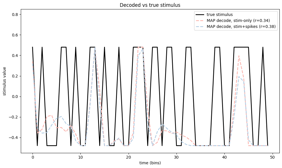
Both decoders recover something of the stimulus. The model conditioned on the actual spike counts typically achieves a higher correlation: it can leverage the real spike history during the test window — refractoriness, bursting, and inter-neuron correlations — in addition to the filter shape, giving it strictly more information than the stimulus-only decoder.
What determines decoding quality?
Several factors trade off here:
Filter quality. A poorly estimated forward filter produces misleading likelihood gradients and degrades the decode regardless of the optimizer.
Smoothness prior strength (\(\lambda\)). Too weak a prior and the optimizer fits noise; too strong and the decoded stimulus is over-smoothed. Here we used the stimulus variance as a data-driven default.
Spike information. Conditioning on the observed spike counts during the test window strictly increases the information available to the decoder, explaining the consistent improvement of the second model.