Tutorial 3+4 - Gaussian and Poisson GLM with Regularization#
Run this tutorial yourself
Download this page as a Jupyter notebook (.ipynb) and run it locally.
This tutorial adapts and combines two notebooks from JW Pillow’s material, presented at the Data Science and Data Skills for Neuroscientists short course at the SfN 2016 meeting:
This is an interactive tutorial designed to walk you through how to fit a GLM while controlling for under/overfitting via regularization and cross-validation. In particular, we will illustrate two forms of regularization: ridge and L2 smoothing.
(Data from Uzzell & Chichilnisky, 2004; see README.txt file in the /data_RGCs directory for details).
The dataset can be downloaded here:
The dataset is provided for tutorial purposes only, and should not be distributed or used for publication without express permission from EJ Chichilnisky (ej@stanford.edu).
Load and pre-process the data#
Below is a quick bit of data wrangling with pynapple that loads and temporally aligns the time series. The final result will be a TsGroup that contains the spike times from 4 RGC units, the corresponding spike counts as a TsdFrame, and a Tsd with the stimulus.
For more details on the pynapple objects and a step-by-step walkthrough of the pre-processing, see the first tutorial.
import matplotlib.pyplot as plt
import numpy as np
from nemos_tutorials import fetch_data, PALETTE, plot_counts
import pynapple as nap
import jax
from scipy.io import loadmat

# enable float64 for precision
jax.config.update("jax_enable_x64", True)

data_paths = fetch_data("data_RGCs")

# Load spike times
spike_times = loadmat(data_paths["SpTimes.mat"], simplify_cells=True)["SpTimes"]
units = nap.TsGroup({i: nap.Ts(val) for i, val in enumerate(spike_times)})

# Load stimulus times and values
stim_times = loadmat(data_paths["stimtimes.mat"], simplify_cells=True)["stimtimes"]
stim = loadmat(data_paths["Stim.mat"], simplify_cells=True)["Stim"]
stimulus = nap.Tsd(stim_times, stim)

# Align time support
units = units.restrict(stimulus.time_support)
Upsample to get finer timescale representation of stim and spikes#
The need to regularize GLM parameter estimates is acute when we don’t have enough data relative to the number of parameters we’re trying to estimate, or when using correlated (eg naturalistic) stimuli, since the stimuli don’t have enough power at all frequencies to estimate all frequency components of the filter.
The RGC dataset we’ve looked at so far requires only a temporal filter (as opposed to spatio-temporal filter for full spatiotemporal movie stimuli), so it doesn’t have that many parameters to estimate. It also has binary white noise stimuli, which have equal energy at all frequencies.
Regularization thus isn’t an especially big deal for this data (which was part of our reason for selecting it). However, we can make it look correlated by considering it on a finer timescale than the frame rate of the monitor. (Indeed, this will make it look highly correlated).
Let’s first restrict all the time series to the first minute — this keeps the notebook fast to run — and then upsample.
# Create a 1min long interval set
epoch_1min = nap.IntervalSet(stimulus.t[0], stimulus.t[0] + 60)

# Restrict the time series
units = units.restrict(epoch_1min)
stimulus = stimulus.restrict(epoch_1min)

# Count with 10x resolution
upsampling_factor = 10
bin_size = (stimulus.t[1] - stimulus.t[0]) / upsampling_factor

# Count the spikes
counts = units.count(bin_size, stimulus.time_support)

# Re-sample the stimulus
stimulus = counts.value_from(stimulus, mode="before")
Pre-processing comparison
Note how the pre-processing pipeline for the upsampled case looks almost identical to the default case by comparing this step with second tutorial. Once the spikes are counted at the right resolution, the re-sampling of other time series is derived from it. No need for special interpolation calls.
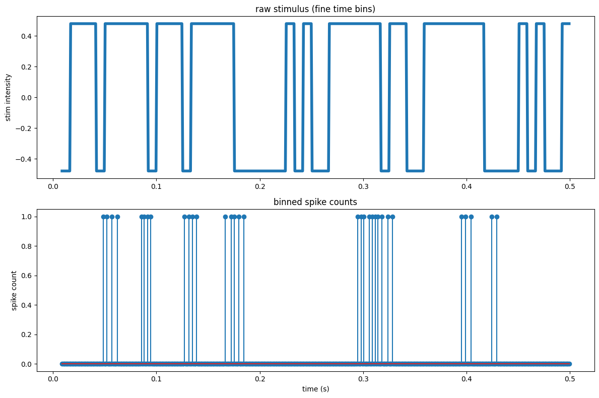
And now let’s visualize the upsampled data.
# Visualize the upsampled data.

fig = plt.figure(figsize=[12,8])
plt.subplot(211)
# plot 0.5 sec
plt.plot(stimulus.get(0, 0.5), linewidth=4)
plt.title('raw stimulus (fine time bins)')
plt.ylabel('stim intensity')
plt.subplot(212)
plt.stem(counts.get(0,0.5).t, counts[:, 2].get(0,0.5).d)
plt.title('binned spike counts')
plt.ylabel('spike count')
plt.xlabel('time (s)')
plt.tight_layout()
plt.show()
Let’s divide in train and test set. This is the simplest way of cross-validating, later we will see improved cross-validation schemes.
# Get the total duration (60 sec)
ep_tot = stimulus.time_support
train_frac = 0.8

train_ep = nap.IntervalSet(
    ep_tot.start,
    ep_tot.start + ep_tot.tot_length() * train_frac
)
# perform a set difference to get the test set
test_ep = ep_tot.set_diff(train_ep)

print("Train:\n", train_ep)
print("\n\nTest:\n", test_ep)
Train:
   index      start      end
      0  0.0083406  48.0083
shape: (1, 2), time unit: sec.


Test:
   index    start      end
      0  48.0083  60.0083
shape: (1, 2), time unit: sec.
Fit the linear-Gaussian model using ML#
As a first step, let’s fit a linear gaussian model without any regularization. We can create the model design as in the first tutorial.
import nemos as nmo

# Define the design matrix
window_size = 20 * upsampling_factor
bas = nmo.basis.HistoryConv(window_size)
X = bas.compute_features(stimulus)
/opt/hostedtoolcache/Python/3.12.13/x64/lib/python3.12/site-packages/pynapple/core/utils.py:198: UserWarning: Converting 'd' to numpy.array. The provided array was of type 'ArrayImpl'.
  warnings.warn(
As in the first tutorial, the HistoryConv columns come in the reverse order from the original notebook; this doesn’t change the model (see the note there), so we flip only when plotting. Since we plot filters repeatedly below, let’s wrap that reordering into a small helper.
def plot_filter(ax, lags, weights, **kwargs):
    # NeMoS' HistoryConv returns the weights with the most recent lag first, so we
    # flip them with [::-1] to align with lag time and match the original notebook.
    ax.plot(lags, weights[::-1], **kwargs)
Now, let’s fit the linear Gaussian model and plot the coefficients.
# Select a cell
cell_idx = 2
neuron_counts = counts[:, cell_idx]

gaussian_glm = nmo.glm.GLM(observation_model="Gaussian", solver_name="BFGS").fit(
    X.restrict(train_ep), neuron_counts.restrict(train_ep)
)

# Plot the coefficients
lags = np.arange(-window_size+1,1) * bin_size
fig, ax = plt.subplots()
plot_filter(ax, lags, gaussian_glm.coef_)
ax.set_title('Fit results')
ax.set_xlabel('time before spike (s)')
plt.show()
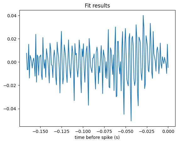
This estimate looks quite noisy. The culprit is that the design matrix is badly conditioned — its singular values span a wide range — which inflates the variance of the unregularized estimate.
To rein in that variance, we turn to regularization.
Ridge regression#
Linear-Gaussian model#
Now let’s regularize by adding a penalty on the sum of squared filter coefficients \(w_i\), of the form
where \(\lambda\) is the “ridge” parameter. This is also known as an “L2 penalty”. Minimizing the error plus this penalty (“penalized least squares”) is equivalent to computing the MAP estimate under an i.i.d. Gaussian prior on the filter coefficients.
For the linear-Gaussian model the MAP estimate has a closed form, making it simple and fast to compute:
The only remaining question is: how to set lambda? We’ll show the simplest way to do so by cross-validation: try a grid of values and pick the one with the best test set score.
Cross-validation schemes
Here we use the simplest possible scheme — a single train/test split. For more robust validation (k-fold, repeated, or stratified splits) reach for the model_selection module of scikit-learn. NeMoS estimators follow the scikit-learn API, so tools like GridSearchCV and KFold work directly on a NeMoS GLM.
NeMoS follows the scikit-learn convention for the ridge penalty, which is scaled a little differently from the original notebook. Before the sweep we therefore re-map the grid of ridge parameters from the original \(\lambda\) to NeMoS’ \(\tilde\lambda = 2\lambda/N\) (see the dropdown below for why).
# Grid matching the original parametrization
lambda_grid = np.logspace(0, 15, 16, base=2)

X_valid = X.dropna()
count_valid = neuron_counts.restrict(X_valid.time_support)
n_samples_train = X_valid.restrict(train_ep).shape[0]

# Re-map to the scikit-learn / NeMoS scaling: lambda_tilde = 2 * lambda / N
lambda_grid *= 2 / n_samples_train
Why the re-mapping?
The original notebook minimizes the summed squared error,
while NeMoS minimizes the averaged squared error,
where \(N\) is the number of (valid) training samples. The only real difference is how the data term is scaled — a sum in \(\mathcal{ll}_o\) versus a per-sample mean in \(\mathcal{ll}_n\). So if we shrink the penalty by the same factor and set
the entire NeMoS objective becomes a constant multiple of the original, \(\mathcal{ll}_n = \frac{2}{N}\,\mathcal{ll}_o\). Scaling an objective by a positive constant never moves its minimum, so the two fits coincide: a ridge parameter \(\lambda\) from the original notebook is exactly \(\tilde\lambda = 2\lambda/N\) in NeMoS.
Let’s cross-validate over the parameter grid, and wrap the procedure into a function that we will re-use later.
def cross_val_model(
    lambdas: np.ndarray,
    design_matrix: nap.TsdFrame,
    y: nap.Tsd,
    train: nap.IntervalSet,
    test: nap.IntervalSet,
    observation_model="Gaussian",
    regularizer="Ridge"
    ):
    n_lambdas = len(lambdas)
    n_coef = X.shape[1]
    coefs = np.zeros((n_lambdas, n_coef))
    intercepts = np.zeros((n_lambdas, ))
    test_scores = np.zeros((n_lambdas, ))
    train_scores = np.zeros((n_lambdas, ))
    for i, l in enumerate(lambdas):
        model = nmo.glm.GLM(
            observation_model=observation_model,
            solver_name="BFGS",
            regularizer=regularizer,
            regularizer_strength=l,
        ).fit(design_matrix.restrict(train), y.restrict(train))
        coefs[i] = model.coef_
        intercepts[i] = model.intercept_[0]
        train_scores[i] = model.score(
            design_matrix.restrict(train),
            neuron_counts.restrict(train)
        )
        test_scores[i] = model.score(
            design_matrix.restrict(test),
            neuron_counts.restrict(test)
        )
    return coefs, intercepts, train_scores, test_scores

coefs, intercepts, train_scores, test_scores = cross_val_model(
    lambda_grid, X, neuron_counts, train_ep, test_ep, regularizer="Ridge"
)
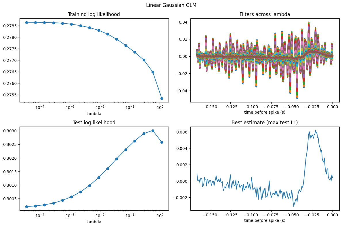
Let’s wrap the four-panel summary into a helper too, since we’ll reuse it for every model below. It shows the train and test log-likelihood across the grid, all the fitted filters, and the filter picked out by the best test score.
def plot_cv_results(lambdas, coefs, train_scores, test_scores, lags, title=""):
    fig, axs = plt.subplots(2, 2, figsize=[12, 8])
    fig.suptitle(title)

    axs[0, 0].set_title("Training log-likelihood")
    axs[0, 0].semilogx(lambdas, train_scores, "-o")
    axs[0, 0].set_xlabel("lambda")

    axs[0, 1].set_title("Filters across lambda")
    for cf, l in zip(coefs, lambdas):
        plot_filter(axs[0, 1], lags, cf, linewidth=4, label=f"lambda: {l:.2e}")
    axs[0, 1].set_xlabel("time before spike (s)")

    axs[1, 0].set_title("Test log-likelihood")
    axs[1, 0].semilogx(lambdas, test_scores, "-o")
    axs[1, 0].set_xlabel("lambda")

    axs[1, 1].set_title("Best estimate (max test LL)")
    plot_filter(axs[1, 1], lags, coefs[np.argmax(test_scores)])
    axs[1, 1].set_xlabel("time before spike (s)")

    fig.tight_layout()
    plt.show()


plot_cv_results(
    lambda_grid, coefs, train_scores, test_scores, lags, title="Linear Gaussian GLM"
)
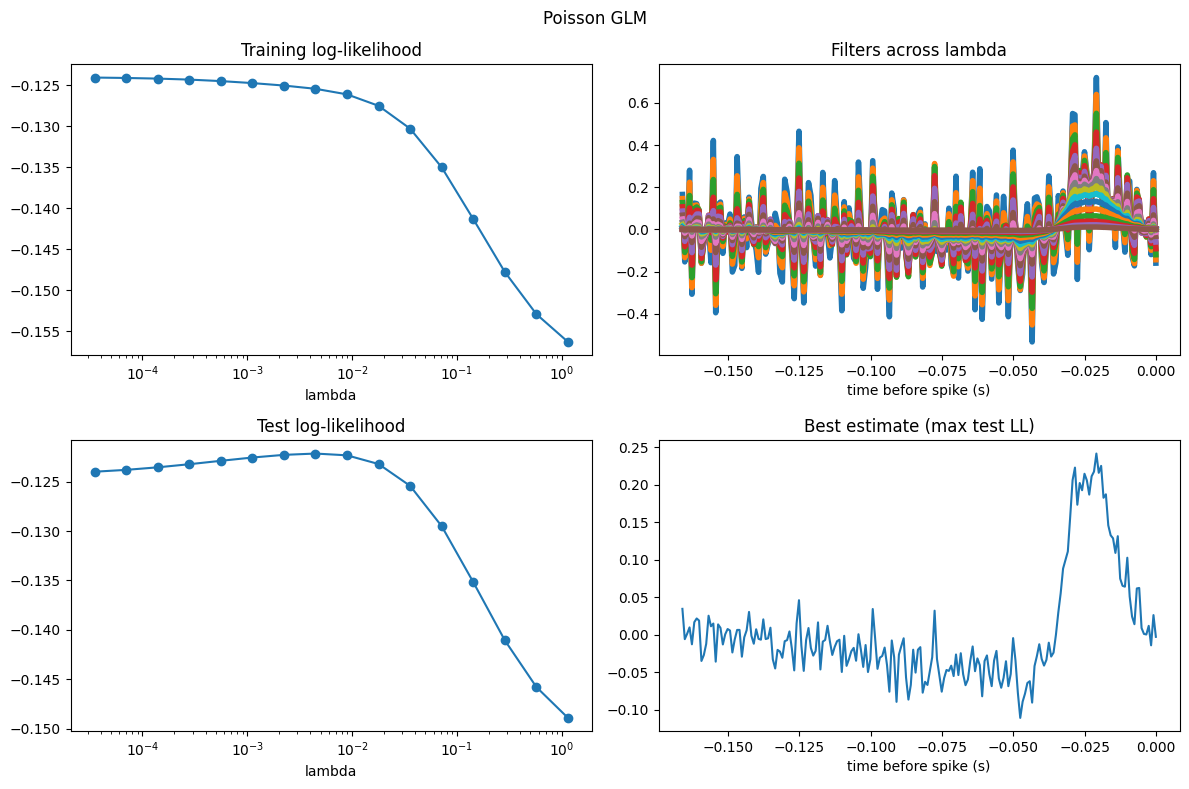
Poisson model#
The Poisson GLM is more of the same: we reuse the exact same cross_val_model, only switching the observation model from "Gaussian" to "Poisson".
coefs_ridge, _, train_ridge, test_ridge = cross_val_model(
    lambda_grid,
    X, neuron_counts, train_ep, test_ep,
    regularizer="Ridge",
    observation_model="Poisson"
)

plot_cv_results(lambda_grid, coefs_ridge, train_ridge, test_ridge, lags, title="Poisson GLM")
NeMoS advanced: L2-smoothing#
So far ridge shrank each coefficient toward zero on its own. A smoothing penalty instead discourages large jumps between adjacent coefficients — a natural prior for a temporal filter, where we expect neighbouring lags to carry similar weight. It penalizes the sum of squared consecutive differences,
NeMoS doesn’t ship this one out of the box, which makes it a good excuse to see how to build a custom regularizer.
From a matrix to a difference#
The original tutorial writes this penalty as a quadratic form \(\mathbf{w}^\top D_x\, \mathbf{w}\), where \(D_x = D^\top D\) is assembled (as a sparse matrix) from the first-difference operator \(D\) — the matrix for which \(D\mathbf{w} = (w_{i+1} - w_i)_i\). But because \(\mathbf{w}^\top D_x \mathbf{w} = \|D\mathbf{w}\|^2\), the whole quadratic form is just the sum of squared differences, and we never need to build \(D_x\) at all: np.diff gives us \(D\mathbf{w}\) directly. Let’s confirm the two agree:
n = X.shape[1]
D = np.diff(np.eye(n), axis=0)   # first-difference operator, shape (n-1, n)
Dx = D.T @ D                     # the "smoothing matrix" of the original tutorial

w = np.random.default_rng(0).normal(size=n)
print("matrix form :", w @ Dx @ w)
print("diff form   :", np.sum(np.diff(w) ** 2))
matrix form : 354.7700298014538
diff form   : 354.7700298014538
Wrapping it as a NeMoS regularizer#
A NeMoS regularizer is a small class. At a minimum you declare which solvers it supports and implement a single method that returns the penalty value; NeMoS takes care of adding it to the loss and optimizing. Two things are worth knowing:
NeMoS applies the penalty only to the regularizable parameters — the coefficients — and leaves the intercept alone. The penalty method just receives those coefficients (and the strength) and returns a scalar.
With several predictors, all their coefficients sit in one stacked vector. We must not smooth across the seam between two different filters, so before differencing we split the coefficients feature-by-feature (this is exactly what
basis.split_by_featuredoes) and penalize each block on its own. Mapping the penalty over that collection of blocks withjax.treeis what lets the very same class handle one predictor or many.
from nemos.regularizer import Regularizer
import jax
import jax.numpy as jnp


class L2Smoothing(Regularizer):
    """L2 smoothing (first-difference) regularizer.

    Penalizes the sum of squared differences between adjacent coefficients,
    ``sum_i (w[i+1] - w[i]) ** 2``, discouraging large jumps and thus
    encouraging smooth filters. This is the quadratic form ``w @ (D.T @ D) @ w``
    with ``D`` the first-difference operator, computed directly from
    ``jnp.diff`` without forming any matrix.

    Parameters
    ----------
    split_fn :
        Callable that splits the coefficient vector into the per-predictor
        blocks that should be smoothed independently (e.g.
        ``basis.split_by_feature``). The penalty is applied to each block and
        summed, so differencing never crosses the seam between two filters.
        Defaults to the identity, i.e. the coefficients are treated as a single
        block — appropriate for a model with a single predictor.
    """

    # solvers this penalty is compatible with
    _allowed_solvers = ["GradientDescent", "BFGS", "LBFGS"]
    # solver used by default
    _default_solver = "BFGS"

    def __init__(self, split_fn=None):
        # splits the coefficients per predictor so we never smooth across
        # filters; think of it as `basis.split_by_feature`
        self.split_fn = split_fn if split_fn is not None else lambda x: x

    @staticmethod
    def smoothness_penalty(coef):
        """Sum of squared differences between adjacent coefficients.

        Equivalent to the quadratic form ``coef @ (D.T @ D) @ coef`` with
        ``D`` the first-difference operator, but without forming any matrix.
        """
        return jnp.sum(jnp.diff(coef, axis=0) ** 2)

    def _penalty_on_subtree(self, subtree, strength, **kwargs) -> jnp.ndarray:
        # NeMoS hands us the regularizable coefficients; split them per
        # predictor, penalize each block, and sum the results.
        par_splits = self.split_fn(subtree)
        penalties = jax.tree.map(
            lambda p: strength * self.smoothness_penalty(p),
            par_splits,
        )
        return jax.tree.reduce(jnp.add, penalties)
With a single predictor the default (no split) is all we need, so we can drop it straight into cross_val_model in place of "Ridge".
reg = L2Smoothing()
coefs_smooth, _, train_smooth, test_smooth = cross_val_model(
lambda_grid,
X, neuron_counts, train_ep, test_ep,
regularizer=reg,
observation_model="Poisson"
)
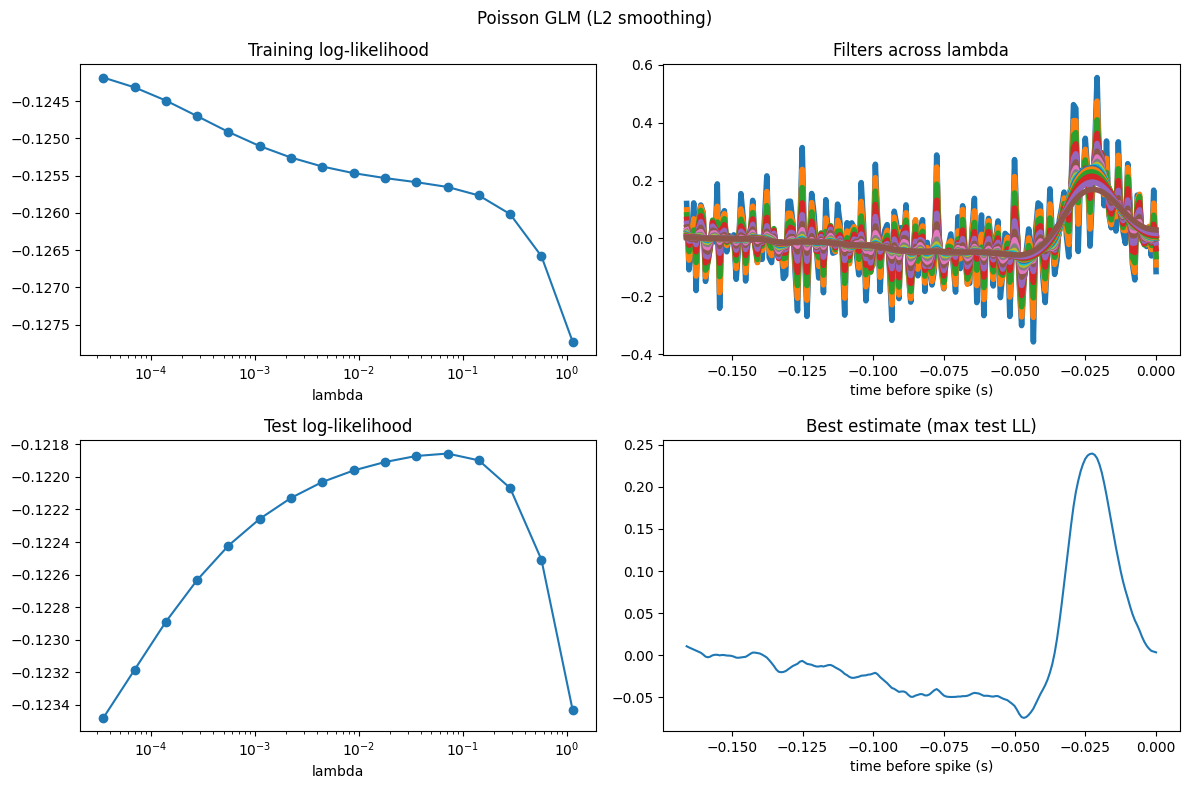
plot_cv_results(
lambda_grid, coefs_smooth, train_smooth, test_smooth, lags, title="Poisson GLM (L2 smoothing)"
)
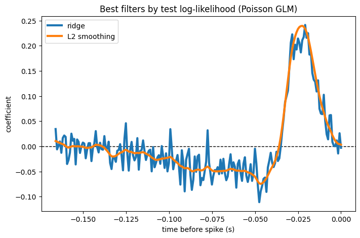
How do the two penalties compare head to head? Let’s pick the best filter under each (the one maximizing test log-likelihood), overlay them, and report their scores.
best_ridge = coefs_ridge[np.argmax(test_ridge)]
best_smooth = coefs_smooth[np.argmax(test_smooth)]

print(f"Best ridge     test LL: {np.max(test_ridge):.5f}")
print(f"Best smoothing test LL: {np.max(test_smooth):.5f}")

plt.figure(figsize=[8, 5])
plt.axhline(0, color="k", linestyle="--", linewidth=1)
plot_filter(plt.gca(), lags, best_ridge, linewidth=3, label="ridge")
plot_filter(plt.gca(), lags, best_smooth, linewidth=3, label="L2 smoothing")
plt.title("Best filters by test log-likelihood (Poisson GLM)")
plt.xlabel("time before spike (s)")
plt.ylabel("coefficient")
plt.legend()
plt.show()
Best ridge     test LL: -0.12216
Best smoothing test LL: -0.12186
Extra: multiple regressors#
There is one thing you don’t want to do with a smoothing penalty: smooth across predictors. When the design matrix stacks several filters end to end, differencing should stay within each filter and never cross the boundary between them. This is exactly what the split_fn is for — we hand L2Smoothing the basis’ split_by_feature, and it penalizes each filter on its own.
window_size_stim = 25 * upsampling_factor
additive = (
    nmo.basis.HistoryConv(window_size, conv_kwargs={"shift": True}, label="spike") +
    nmo.basis.HistoryConv(window_size_stim, label="stim")
)
X_multi = additive.compute_features(stimulus, neuron_counts)

reg_multi = L2Smoothing(lambda x: additive.split_by_feature(x, axis=0))
model = nmo.glm.GLM(regularizer=reg_multi)
model.fit(
    X_multi.restrict(train_ep),
    neuron_counts.restrict(train_ep)
)
/opt/hostedtoolcache/Python/3.12.13/x64/lib/python3.12/site-packages/pynapple/core/utils.py:198: UserWarning: Converting 'd' to numpy.array. The provided array was of type 'ArrayImpl'.
  warnings.warn(
/opt/hostedtoolcache/Python/3.12.13/x64/lib/python3.12/site-packages/pynapple/core/utils.py:198: UserWarning: Converting 'd' to numpy.array. The provided array was of type 'ArrayImpl'.
  warnings.warn(
GLM(
    observation_model=PoissonObservations(),
    inverse_link_function=exp,
    regularizer=L2Smoothing(split_fn=<function <lambda> at 0x7f8a3bbc6a20>),
    regularizer_strength=1.0,
    solver_name='BFGS'
)
In a Jupyter environment, please rerun this cell to show the HTML representation or trust the notebook. On GitHub, the HTML representation is unable to render, please try loading this page with nbviewer.org.
Parameters
| observation_model | PoissonObservations() | |
| inverse_link_function | <function exp...x7f8a6415ce00> | |
| regularizer | L2Smoothing(s...7f8a3bbc6a20>) | |
| regularizer_strength | 1.0 | |
| solver_name | 'BFGS' | |
| solver_kwargs | {} | |
| regularizer__split_fn | <function <la...x7f8a3bbc6a20> |
Fitted attributes
| Name | Type | Value |
|---|---|---|
| aux_ | NoneType | None |
| coef_ | ArrayImpl[float64](450,) | Array([ 0.033...dtype=float64) |
| dof_resid_ | ArrayImpl[float64](1,) | Array([57549.], dtype=float64) |
| intercept_ | ArrayImpl[float64](1,) | Array([-2.997...dtype=float64) |
| scale_ | ArrayImpl[float64](1,) | Array([1.], dtype=float64) |
| solver_state_ | OptimistixAdapterState | OptimistixAda...k_bool[] ) ) |
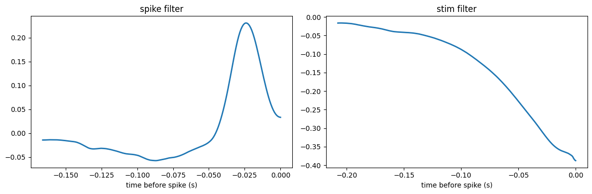
The same split_by_feature we passed to the regularizer also lets us pull the two filters back out of the fitted coefficients and plot each one — smoothed within itself, never across the seam.
filters = additive.split_by_feature(model.coef_, axis=0)

fig, axs = plt.subplots(1, len(filters), figsize=[12, 4])
for ax, (label, filt) in zip(axs, filters.items()):
    filt = np.asarray(filt).squeeze()
    lag = np.arange(-filt.shape[0] + 1, 1) * bin_size
    plot_filter(ax, lag, filt, linewidth=2)
    ax.set_title(f"{label} filter")
    ax.set_xlabel("time before spike (s)")
fig.tight_layout()
plt.show()
Regularizers shipped with NeMoS#
We built L2Smoothing by hand because NeMoS doesn’t ship it, but several common regularizers come built in. As of NeMoS v0.2.7 you can pass any of the following as regularizer= (by name, e.g. "Ridge", or as an instance):
Regularizer |
Penalty |
What it does |
|---|---|---|
|
\(\tfrac{\alpha}{2}\lVert w\rVert_2^2\) |
L2 shrinkage toward zero (MAP under an i.i.d. Gaussian prior); the workhorse used above. |
|
\(\alpha\lVert w\rVert_1\) |
L1 penalty; promotes sparsity, driving some coefficients exactly to zero. |
|
\(\alpha\big(\rho\lVert w\rVert_1 + \tfrac{1-\rho}{2}\lVert w\rVert_2^2\big)\) |
Convex mix of L1 and L2 — sparsity with the grouped shrinkage of ridge. |
|
\(\alpha\sum_g \lVert w_g\rVert_2\) |
L1 across predefined groups of coefficients; selects or zeros out whole groups (e.g. all weights of one feature) at once. |
In every case the intercept is left unpenalized, and the strength is set through regularizer_strength (the \(\alpha\) above). For anything not on this list — like our smoothing penalty — you subclass Regularizer, exactly as we did.